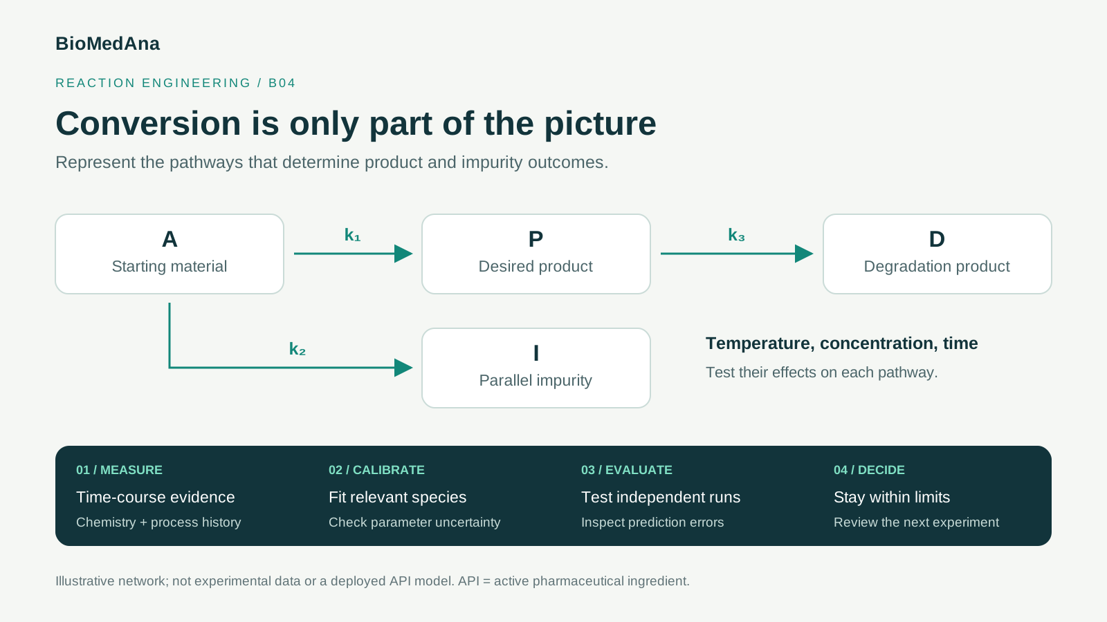
Reaction kinetics modeling in pharmaceutical development uses rate laws and material balances to describe how reactants, products, and impurities change over time. For active pharmaceutical ingredient (API) processes, it helps teams test how temperature, concentration, and addition profiles could affect conversion and selectivity. Useful predictions require suitable measurements, parameter calibration, independent evaluation, and explicit limits on where the model applies.
A reaction reaches the conversion target sooner at a higher temperature. The impurity result is worse. Should the team lower the temperature, change the addition profile, or shorten the hold?
A kinetic model gives process chemists, process development (PD) teams, and modelers a way to examine those choices together. Its purpose is to connect a proposed operating change to measurable consequences and identify the experiment that should test the prediction.
This guide focuses on chemically synthesized APIs. The equations and example below are illustrative; they are not a deployed BioMedAna API model or a customer result.
What decision should a reaction kinetics model support?
Start with one decision and the outputs needed to make it. “Model the reaction” is too broad. “Compare two addition profiles against conversion and a specified impurity at the end of the hold” defines a useful scope.
Record the operating range, measured species, relevant equipment, and acceptable prediction error before fitting. A model intended to estimate reaction time may need different evidence from one used to predict a low-level impurity.
For broader context on connecting a process model to new observations, see What Is an API Digital Twin? Applications in Development, Scale-Up and Manufacturing.
How do you choose a rate law?
A common starting form is:
Here, is reaction rate per unit volume, and are concentrations, is a temperature-dependent rate coefficient, and and describe the concentration dependence. For this form, the overall reaction order is . The orders must be supported by evidence; they cannot generally be read from the balanced overall reaction. IUPAC: order of reaction
Keep units explicit. With concentrations in mol/L and time in minutes, a first-order coefficient has units min⁻¹; a second-order coefficient has units L mol⁻¹ min⁻¹.
A simple power law may be an adequate local description. Reversibility, catalyst deactivation, inhibition, or changing speciation may require a different expression. A good fit alone does not prove a molecular mechanism.
Reaction-progress analysis can help distinguish candidate explanations. In a published primary study of palladium-catalyzed arylation, researchers used reaction-progress kinetic analysis to explore substrate dependence and guide catalyst development. That is a specific research application, not evidence that one rate expression works across pharmaceutical reactions. Primary research study
How do competing reactions change the answer?
Conversion measures consumption of starting material; it does not establish how much desired product formed. Consider an illustrative irreversible network:
is the desired product, a parallel impurity, and a degradation product. For a well-mixed, constant-volume batch with first-order steps:
These equations assume a closed, single-phase system, one-to-one stoichiometry, and no other reactions. Their sum is zero, conserving the modeled A-derived material. Real chemistry may need additional species and balances.
The network exposes two different trade-offs: A can form I instead of P, and P can degrade while the batch waits. Parallel and series reactions therefore need separate treatment when evaluating selectivity and hold time. University of Michigan: multiple reactions
For a deliberately simplified numerical illustration, set , min⁻¹, and min⁻¹, with only A initially present. At 90% A conversion, the elapsed time is minutes. P yield on initial A is 75%, while I yield is 15%. The remaining 10% is A. These are calculated values from invented coefficients, not experimental data.
One useful limitation follows directly: when both parallel steps are first order in A at fixed temperature, reducing A concentration changes both rates proportionally and does not change their rate ratio. A slower feed is therefore not automatically more selective. It may help in a different network, under different reaction orders, or by changing thermal or local mixing conditions—effects that need their own evidence.
What data are needed for a useful kinetic model?
Collect time-resolved chemistry and the process history that produced it. An endpoint assay alone rarely distinguishes competing rate laws.
| Data | What to record | Why it matters |
|---|---|---|
| Concentration profiles | Starting material, product, relevant impurities, timestamps, units, analytical uncertainty | Separates consumption from formation and degradation |
| Temperature history | Measured reaction temperature, ramps, excursions, probe location | A jacket setpoint is not necessarily the reacting mixture temperature |
| Charges and feeds | Initial amounts, concentrations, actual feed histories, sampling losses, volume changes | Reconstructs the material balance |
| Chemical context | Solvent composition, water, catalyst loading, material lots, relevant pH or acidity | Helps identify conditions that alter apparent kinetics |
| Physical context | Agitation, phases, solids, pressure, gas supply, equipment | Helps distinguish chemical kinetics from transport limitations |
| Measurement context | Calibration, response factors, quantitation limits, sampling and quench procedure | Prevents analytical artifacts from becoming fitted chemistry |
Chromatographic area percentages should not automatically be treated as molar concentrations. Establish a suitable quantitative basis and account for response differences. An impurity reported below its quantitation limit is not necessarily absent.
Design experiments to separate effects: vary initial concentrations independently where practical, study multiple temperatures, and include holds that can reveal product degradation. Replicates help estimate variability. Dense sampling from one run adds trajectory detail but does not replace independent runs across the proposed operating range.
There is no universal minimum number of experiments. The requirement depends on model complexity, measurement quality, and whether the chosen conditions distinguish the parameters that matter to the decision.
How should the model be calibrated and checked?
Calibration estimates parameters from data. Independent evaluation tests whether those fitted parameters support the intended prediction. The following workflow is a practical editorial proposal for scientific review.
- Verify the balances and implementation. Check stoichiometry, units, initial conditions, numerical tolerances, and material conservation. For semibatch operation, use a balance such as , with any additional relevant sources or losses. Here, is liquid volume, is volumetric flow, and is the signed stoichiometric coefficient of species i in reaction j. The outlet term assumes the exiting fluid has the bulk composition. Do not reuse constant-volume concentration equations without accounting for dilution.
- Fit relevant species and experiments together. Integrating the balance equations and fitting concentrations avoids directly differentiating noisy concentration measurements. Use an objective and weighting appropriate to the measurement-error model; otherwise, a high-concentration species can dominate the result.
- Inspect parameter stability. Try credible starting values and examine correlations and sensitivity. Nonlinear optimization can converge to local minima, and outliers can materially affect estimates. NIST: nonlinear least squares
- Look at residuals, not only a fit statistic. Plot measured-minus-predicted values against time, temperature, concentration, and experiment. Persistent structure suggests a missing effect or measurement problem. NIST: assessing model fit
- Test independent runs. Reserve entire experiments for evaluation, including conditions relevant to the decision. Randomly splitting adjacent samples from the same run can overstate predictive performance.
- Assess uncertainty against the decision. Examine whether plausible parameter and measurement variation changes the preferred condition. Prediction intervals based on a chosen model do not automatically cover missing pathways or new physical regimes.
For the illustrative network, measuring A alone identifies the sum , not each coefficient separately. Measuring P and I can help resolve that ambiguity. This is an identifiability issue: more optimizer iterations cannot replace missing information.
If several parameter sets fit equally well but recommend different operating conditions, the next deliverable should be a discriminating experiment rather than an apparently precise operating recommendation.
What does the Arrhenius equation tell you?
The Arrhenius equation relates a rate coefficient to absolute temperature:
is the pre-exponential factor, the activation energy, the gas constant, and temperature in kelvin. The original form treats and as temperature-independent. IUPAC: Arrhenius equation
A convenient equivalent form for fitting is:
Use consistent energy units: for example, J mol⁻¹ K⁻¹ requires in J/mol. Estimate temperature dependence over a relevant range; two fitted rate coefficients can define a line without adequately testing whether that relationship remains useful.
Each pathway may have a different temperature dependence. In the illustrative parallel network, if the impurity pathway has a larger activation energy than the desired pathway, increasing temperature increases , assuming both retain Arrhenius behavior. Faster conversion can then come with poorer branching selectivity. Product degradation adds another time-dependent trade-off.
Treat departures from the fitted relationship as a prompt to investigate changes in chemistry, phases, or transport. Extending an Arrhenius curve beyond the evaluated range does not establish that the extrapolation is valid.
Where do reaction kinetics models stop being reliable?
A model’s usable range includes chemical and physical conditions, not just temperature limits. Record solvent composition, concentration, catalyst state, phases, material attributes, equipment assumptions, and the outputs evaluated.
A fitted coefficient may describe apparent behavior influenced by mixing, gas–liquid transfer, or dissolution. Transferring that coefficient to a different reactor can fail even if the laboratory concentration profiles were reproduced well.
For scale-up, evaluate whether mixing and transport remain fast enough relative to reaction, whether local feed concentrations matter, and whether heat removal changes the temperature history. Thermal predictions require reaction enthalpies and energy balances; safety assessment also requires suitable calorimetry and consideration of hazardous pathways beyond the fitted network.
The model should be reconsidered when a new impurity appears, material-balance closure deteriorates, a phase changes, or independent runs show systematic error. An omitted impurity cannot be assumed to remain controlled because the main reaction is well fitted.
How can a kinetics study start a Bio Twin conversation?
A kinetic model can become one component of a broader process representation. BioMedAna Twin publicly describes predictive simulation and scenario comparison around process evidence and review. Its bioprocess positioning does not by itself establish a deployed synthetic API kinetics capability.
For a synthetic API project, begin with the reaction decision, available analytical profiles, candidate pathways, and the conditions under which predictions would be used. Agree on the evidence a focused feasibility study would need to produce.
Bring one reaction, one conversion or impurity question, and the available time-course data to a technical conversation about Bio Twin. Define what a useful model would need to explain—and how you would test it.
Frequently asked questions
What is reaction kinetics modeling in pharma?
Reaction kinetics modeling uses rate laws and material balances to describe how reactants, products, and impurities change over time. In pharmaceutical process development, it supports questions about reaction time, temperature, addition profiles, and selectivity within a defined range of conditions.
What data are needed to build a reaction kinetics model?
Typically, teams need time-resolved concentrations, actual temperature and feed histories, initial charges, volume information, and analytical uncertainty. Solvent, catalyst, material, and mixing context help determine whether apparent behavior reflects chemical kinetics or other effects.
Can reaction kinetics modeling predict impurities?
It can estimate a specified impurity when the relevant formation and consumption pathways are represented and supported by suitable measurements and independent evaluation. A model of starting-material disappearance alone does not establish impurity predictability.
How many experiments are needed for kinetic modeling?
There is no fixed number. Experiments must distinguish relevant parameters, cover the proposed conditions, characterize variability, and provide independent evaluation. Many samples from one batch cannot substitute for that experimental coverage.
Does a higher reaction temperature improve yield?
Not necessarily. Temperature may accelerate desired and undesired pathways differently. Higher conversion can coincide with more impurity formation or product degradation, so yield and selectivity must be evaluated alongside reaction time.
What is the difference between calibration and validation?
Calibration fits model parameters to observations. Validation evaluates fitness for a stated use against defined criteria and appropriate evidence, including independent experiments. A close fit to calibration data alone does not establish reliable prediction or scale-up performance.